Temporal Variance Contrast Analyzer
Description
Motivation
High-contrast performance is one of the prime metrics to judge the quality of closed-loop operation of AO systems these days. Thus, a contrast curve must not be missing from any decent analysis tearsheet for a give AO simulation.
The prime motivations to come up with TVC was the following list of requirements: Computing the TVC should allow to
- be able to quickly access the contrast of a large set of simulations (hundreds) that produced a large number of residual WF frames (thousands) each.
- not have to rely on specific assumptions about position in the sky, amount of field rotation, ADI algorithm used, etc.
- assess essentially the impact of a given deterioration of wavefront quality, rather than the precise value.
No. 1 inhibits the use of a full-fledged analysis software like such as VIP ([GomezGonzales+2017] ), which usually runs a couple of hours on each simulation output. We needed something much simpler and faster.
No. 2 fostered the idea of coming up with a measure that attempts a measurement of those limitations that any ADI algorithm would be unable to overcome. This has only partly been achieved, but the underlying thoughts are: Static aberrations cause static PSF patterns, which are easy to handle and cause little or no noise. Aberrations that are de-correlated between frames cause independent realizations of random PSF patterns, these can essentially not be overcome by ADI methods (But instead average out to a certain degree over time). That leaves aberrations that change in intermediate time-scales for the ADI algorithms to handle. These, however, are hardly present in our simulations as we do not simulate NCPA variations, flexure, pupil shifts, or any other slow effect yet.
So in order to measure the fundamental limit imposed by the independent realizations, we came up with the idea of looking at the variance along the temporal axis at each image location separately. This is nicely independent of any assumed amount of field rotation, which would not change these statistics. As variance can be computed in an on-line fashion on focal-plane frames being computed one-by-one subsequently, the method is suitable to operate on very large data sets that can not be held in memory entirely. Since we are not heavily interested in the absolute contrast value, we operate on single pixels only rather than averaging over a certain aperture.
Definition
For this section, we compute a comparison between TVC and a standard ADI contrast. We use a simulation data set from the METIS ([Brandl+2018] ) preliminary design phase.
We define two types of contrast to compare, in addition to the actual HCI result. First the TVC. It is computed in the following way:
- Compute image frames from the residual phases and stack in a cube
- Compute the variance \(V\) along the temporal axis for each pixel
- For a give separation, average the variances over an annulus covering that separation
- Compute the 5σ contrast for that separation as as \(5 \times \sqrt{V}\)
In order to have a simplified model for ADI, we compute what we will call the ADI contrast in the following way
- Compute image frames from the residual phases and stack in a cube
- Compute a robust mean image along the temporal axis, robust meaning we exclude the 10% of values furthest from the median in each temporal vector.
- Subtract the above image from each frame
- Average along the temporal axis
- For a given separation, compute the variance \(V\) of pixel values over an annulus covering that separation
- Compute the 5σ contrast for that separation as as \(5 \times \sqrt{V}\)
Note that when the assumption works that the temporal variance is a good measure for the variations that cannot be overcome by the ADI algorithm, the TVC contrast and the ADI contrast computed in this way should be related by the square root of the number frames. This is because the ADI procedure averages along the temporal axis, and the error of the mean (found in the spatial standard deviation when ADI contrast is measured) should be given by the temporal standard deviation divided by the square root of the number of independent realizations.
Comparison to ADI
In order to compare the various methods to measure contrast, we computed the TVC and the above simplified ADI model on the same residual phase cube that was used to derive the contrasts in the METIS PDR.

Contrast curves measured on the standard HCI data set. The green curve is the actual ADI result obtained by running VIP ([GomezGonzales+2017] ) on the resulting image cube. The straight blue line represents the ADI contrast measured with the method defined in Sec. Definition. The dotted blue line is the same divided by the square root of the number of frames in the cube. The orange curve represents our simplified ADI model, also defined in Sec. Definition.
The above figure shows the contrast curves derived in the various ways. Two observations can be made.
Firstly, the match of the TVC curve divided by the square root of the number of frames to the
contrast curve measured by true ADI via the VIP package is excellent. Note that in the cube used
as input for this experiment is sampled at 300 ms steps, all frames are completely
de-correlated from one another. tvc_analyzer tries to determine the correlation length of a given input cube, and divide by the
number of independent realizations instead of the number of frames in order to predict final 1hr ADI contrast. If this determination goes wrong for some reason, results can become unreliable!
The temporal statistics do not vary with time in these simulations - the TVC contrast measured on 500 frames is the same as the one measured on the full set of 12,000 frames. Thus, if the condition of independent frames and no mid-temporal-frequency being present in the system is granted, the analysis can be greatly accelerated by running only on a subset!
Secondly, the simplified ADI model matches the scaled TVC and the measured ADI curve only partly. While the match in the interesting region around \(5λ/D\) is reasonable, the curves diverge around the control radius. It is beyond the scope of this comparison to investigate the details of this behaviour.
Impact of wavefront quality
While the prediction of the actual high-contrast performance is nice-to-have, the prime goal of a contrast analysis in AO simulations is to catch all factors that have a pronounced impact on the high-contrast performance of the system.
In order to investigate this, we deteriorated the wavefronts by multiplying residual phase screens with a factor. The impact on contrast at 5λ/D can be seen in the figure below:

Evolution of contrast versus wavefront quality.
TVC and modeled ADI contrast as defined in Sec. Definition behave nicely in parallel. The exact factors found are listed in the table below:
| Contrast loss factor | ||
|---|---|---|
| Wavefront rms [nm] | ADI model | TVC model |
| 91.1 | 1.00 | 1.00 |
| 96.6 | 1.10 | 1.10 |
| 111.0 | 1.21 | 1.20 |
| 115.0 | 1.31 | 1.31 |
| 129.1 | 1.42 | 1.41 |
| 137.9 | 1.52 | 1.51 |
| 141.2 | 1.63 | 1.62 |
| 151.8 | 1.74 | 1.73 |
| 157.8 | 1.85 | 1.84 |
| 162.4 | 1.97 | 1.94 |
TVC appears to be slightly less impacted than the ADI model, but not to the level accuracy used in this report. We conclude, that we can safely use our TVC analyses to find critical impacts on contrast caused by the topics under analysis in this report. The impact factors and the resulting budget should be representative for the full HCI analysis using state of the art ADI algorithms.
tvc_analyzer
tvc_analyzer is different from ost other analyzers in AOSAT as it can run in two distinct mode: Coronagraphic and non-coronagraphic. Thisis selected during instantiation by means of the ctype keyword:
a = tvc_analyzer(ctype='icor') # run with an ideal (perfect) coronagraph inserted
a = tvc_analyzer(ctype='nocor') # run without coronagraph
a = tvc_analyzer()              # run without coronagraph
When running in coronagraphic mode, the PSF creation from each residual phase frame is routed through a perfect coronagraph as described in [Cavarroc+2005] .
In this case, the incoming complex amplitude \(A\) (represented as tel_mirror * exp(1j*phase)) is modified to \(\bar{A} = A - \Pi\), where \(\Pi\) repreesents the telescope pupil. The usual factor of a square root of Strehl \(\sqrt{S}\) is not implemented in tvc_analyzer, as Strehl is either so high that it’s negligible, or the determination of \(S\) is unreliable. Thus the implementation is tel_mirror * exp(1j*phase) - tel_mirror.
In addition, tvc_analyzer produces an additional plot by default when instantiated in coronagraphic mode: The coronagraphic PSF.
Plot captions
When called on its own in coronagraphic mode, or on a figure with sufficient available subplot space, tvc_anaylzer.makeplot() will produce two figures like so:
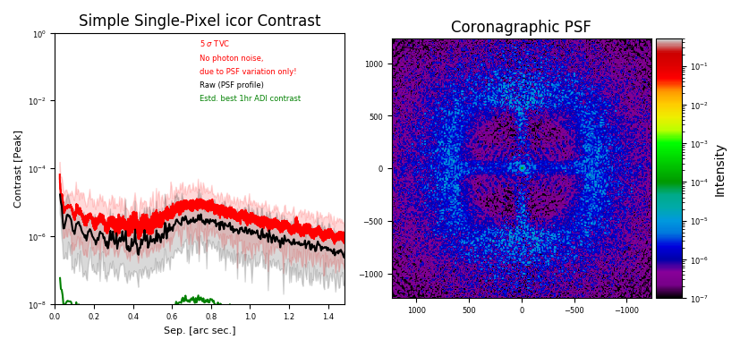
The figure caption for the left image would be :
Resulting contrast curves. The black curve shows the PSF profile, the red curve the resulting :math:`5sigma` contrast from temporal variation of the PSF. The green curve shows the predicted contrast limit achievable in an integration of 1hr after ADI processing.
The figure caption for the right image would be :
Time-averaged coronagraphic PSF. Intensities are relative to the peak of the non-coronagraphic PSF.
In the non-coronagraphic case, the right figure is missing. The green curve is plotted only if a successful determination of the correlation time could be achieved.
Resulting properties
tvc_analyzer exposes the following properties after finalize() has been called:
| Property | type | Explanation |
|---|---|---|
ctype |
str | type of coronagraph (“icor” or “nocor”) |
mean |
2D ndarray | time-averaged PSF. |
variance2: 2D ndarray |
variance2[1] contains the non-coronagraphic time-averaged PSF (icor only) | |
contrast |
2D ndarray | 5 sigma contrast of the PSF |
rcontrast |
2D ndarray | raw contrast, i.e. the normalized PSF. |
rvec |
2D ndarray (float) | Image where each pixel contains distance to centre (mas) |
cvecmean |
2D ndarray (float) | Mean TVC contrast at locatstepoions in rvec. |
cvecmin |
2D ndarray (float) | Minimum TVC contrast at locations in rvec. |
cvecmax |
2D ndarray (float) | Maximum TVC contrast at locations in rvec. |
rvecmean |
2D ndarray (float) | Mean raw contrast at locatstepoions in rvec. |
rvecmin |
2D ndarray (float) | Minimum raw contrast at locations in rvec. |
rvecmax |
2D ndarray (float) | Maximum raw contrast at locations in rvec. |
corrlen |
float | Measured correlation length [#frames] |
max_no_cor |
float | Peak intensity of non-coronagraphic PSF |
Note that currently 2D array can be either numpy or a cupy NDarray, depending on whether CUDA support is used or not. When feeding those to other libraries, such as matplotlib, you are advised to use aosat.util.ensure_numpy(array).
References
| [Brandl+2018] | SPIE 10702, Status of the mid-IR ELT imager and spectrograph (METIS) |
| [Cavarroc+2005] | A&A 447, 397, Fundamental limitations on Earth-like planet detection with extremely large telescopes <https://ui.adsabs.harvard.edu/link_gateway/2006A&A…447..397C/arxiv:astro-ph/0509713> |
| [GomezGonzales+2017] | (1, 2) The Astronomical Journal 154(1), VIP: Vortex Image Processing Package for High-contrast Direct Imaging |