Spatial Power Spectrum Analyzer
Description
The power spectrum analyzer derives the time-averaged spatial power spectrum of the residual phase frames.
Anti-aliasing
The spatial power spectrum is derived by an FFT of the input residual phase:
fftArray       = np.fft.fftshift(np.fft.fft2(ps*mask,norm='ortho'))
fftArray       = (fftArray * np.conj(fftArray)).astype(np.float)
The mask deployed here is an apodized version of the input pupil. The apodization avoids ringing, i.e. the appearance of Airy-ring-like structures in the power spectrum. Apodization is achieved by modifying the input telescope pupil mask in three steps:
- transfor it into a pure binary mask
- apodize the binary mask by applying skimage.morphology.binary_dilation 3 times to derive 3 versions of the pupil, each 1 pixel smaller than the previous one.
- The 1 pixel wide border region which makes the difference between successively dilated pupils is assigned a transmission value according to a Gaussian fall-off.
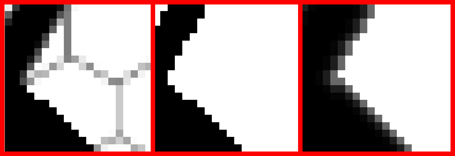
Pupil apodization. Left: crop of the original telescope pupil, in this case of the ELT showing a representation of the segmentation. Center: Same crop of the pupil after “binarization”. Right: Apodized pupil applied to residual phase to avoid aliasing/ringing.
Currently there is no parameter to vary the number of steps for the apodization. In case you absolutely want to, you’d have to assign the mask manually like so:
>>> import aosat
>>> nsteps = 6 # let's say you ant 6 steps for a really soft pupil
>>> a=aosat.analyze.sps_analyzer()
>>> a.mask = util.apodize_mask(a.sd['tel_mirror'] != 0,steps=nsteps)
The resulting power spectra are averaged azimuthally, and finally temporarily.
Plot captions
When called on its own mode, or on a figure with sufficient available subplot space, make_plot() will produce a figure like so:

The figure caption would be:
time-averaged spatial power spectrum of the residual wavefronts. For comparison, the red line shows the expected open-loop Kolmogorov spectrum. The blue line represents a von Kármán spectrum for an outer scale of \(L_0=25\) m.
Note that the blue line is plotted only, when the L0 key is present in the setup dictionary
Resulting properties
sps_analyzer exposes the following properties after finalize() has been called:
| Property | type | Explanation |
|---|---|---|
mask |
2D ndarray (float) | Apodization mask generated from puppil |
f_spatial |
1D ndarray (float) | Spatial frequency vector [1/m] |
ps_psd |
1D ndarray (float) | Power spectral density at f_spatial [nm^2/m^-1] |
Note that currently 2D array can be either numpy or a cupy NDarray, depending on whether CUDA support is used or not. When feeding those to other libraries, such as matplotlib, you are advised to use aosat.util.ensure_numpy(array).